Enterprise data engineering rarely fails because of missing tools. It fails because of constraints that nobody can change. One of the most common constraints is source query row limits. Legacy databases, third-party systems, and APIs often restrict how many rows can be returned on a single request.
When a data platform scales, these limits stop being minor inconveniences and start blocking production pipelines. Instead of fighting the limitation, the solution is to design around it. This article walks through a practical, reusable partition pipeline pattern in Microsoft Fabric that allows large tables to be loaded safely and systematically, even when the source system imposes strict row limits.
Understanding the Problem: Why Row Limits Exist
Before we jump into solutions, let’s understand why these limits exist. These limits are typically introduced to protect system stability, manage resource consumption, and control operational cost.
Common reasons for query row limits:
- Resource Protection: Prevents a single query from exhausting memory or CPU.
- Network and Throughput Control: Avoids excessive data transfer in a single call.
- Legacy System Stability: Older systems often cannot handle modern data volumes.
- Cost Governance: Many platforms charge based on data extraction volume.
Whatever the reason, you’re stuck with it. Complaining to the DBA won’t help. Asking for an exception won’t work. You need a different approach.
That’s where partition pipelines come in. Instead of fighting the limit, we’ll work with it by breaking our data load into bite-sized pieces.
The Solution: Partition Based Data Loading
From an enterprise perspective, partition pipelines are not only a technical optimization. They are also a governance mechanism that protects source systems and controls operational risk.
The core idea is simple: if you can’t load all your data in one query, split it into multiple smaller queries. Each query stays under the row limit, and together they get you all the data you need. This pattern is not a workaround. It is a scalable data engineering design principle that can be reused across multiple workloads and environments.
Here’s how the entire process will work:
- Analyze your data to find a good partition column (usually a date column)
- Determine the right partition granularity (year, month, or day)
- Build a pipeline that loops through each partition
- Load each partition separately, keeping under the row limit
For example, if your sales table has 4 million rows and your source limits you to 500K rows, you might partition by month. Each month’s data becomes a separate query, and you load 12 months one at a time.
Step 1: Analyze Your Source Data
The first step is understanding your data distribution. You need to know:
- Total row count on your source table
- Which column to use for partitioning (typically a date or timestamp)
- How rows are distributed across time periods
Choosing the Right Partition Granularity
Let’s say your source database has a 500,000-row limit. You have three years of transaction data in a table called FactSales. Here’s how to decide your partition strategy:
Option 1: Partition by Year
First, check how many rows each year contains:
| Period | Total Rows |
| 2007 | 4,000,025 |
| 2008 | 3,626,523 |
| 2009 | 5,001,060 |
Problem: Every year exceeds 500K rows. Partitioning by year won’t work. We need finer granularity.
Option 2: Partition by Year-Month
Let’s go one level deeper and check monthly row counts: Here I have attached few months total row counts to get a clear idea.
| Period | Total Rows | Status |
| 200701 | 356,858 | ✓ OK |
| 200907 | 484,401 | ⚠ Close |
| 200912 | 478,320 | ⚠ Close |
Good news: All months are under 500K rows. Monthly partitioning will work.
However, if you notice that July 2009 has 484,401 rows dangerously close to the limit (500,000). If business grows, you might exceed 500K in future months. This brings us to a critical decision point.
Option 3: Partition by Year-Month-Day (Future-Proof)
For a future-proof solution, consider going to one more level deeper daily partition. Yes, this creates more partitions (about 1,095 days for three years), but each day’s data will be well below the limit:
| Period | Total Rows |
| 20070101 | 11,242 |
| 20070102 | 11,371 |
| 20070103 | 12,023 |
Decision Guidelines:
- Use monthly partitions if all months are comfortably under the limit (< 70% of max)
- Use daily partitions if any month approaches the limit or if you expect data growth
Choosing the correct granularity directly impacts how well your pipeline will scale as data volumes increase over time.
Helping Query: Getting Row Counts
Use this SQL query to analyze your data distribution:
— For monthly analysis
SELECT
FORMAT(DateColumn, ‘yyyyMM’) AS Period,
COUNT(*) AS TotalRows
FROM FactSales
GROUP BY FORMAT(DateColumn, ‘yyyyMM’)
ORDER BY Period;
Step 2: Set Up Data Gateway Connection
If your source is an on-premises SQL Server (like the Contoso database in this example), you need to set up an on-premises data gateway. If you’re using a cloud data source, you can skip this step.
Install and Configure the Gateway
- Download and install the On-Premises Data Gateway from Microsoft
- Register the gateway with your Microsoft account
- Create a connection in Fabric that uses this gateway
Creating the Connection:
- Go to your Fabric workspace settings
- Navigate to Data Gateway → Connections
- Click ‘New’ and select ‘SQL Server’
- Enter your server’s name and database name
- Provide SQL Server authentication credentials (username and password)
- Name your connection (e.g., ‘Local DB Conn’)
Once created, open the connection properties and copy the Connection ID. You’ll need this for your pipeline parameters.
Important: Your SQL Server must be configured for SQL Server Authentication (not just Windows Authentication) for the gateway connection to work. Ask your DBA if you’re unsure.
Step 3: Build the Partition Pipeline
Now comes the fun part of building the actual pipeline. We’ll make this dynamic and reusable so you can use the same pipeline with small enhancements for multiple tables.
Create the Pipeline and Define Parameters
Step by step:
- In your Fabric workspace, click ‘New’ → ‘Data Pipeline’
- Give a name example ‘PL_Load_Fact_Table_By_Partition’
- Click on the blank canvas, then click ‘Parameters’ in the bottom panel
Create these parameters to make your pipeline dynamic:
| Parameter | Type | Purpose |
| Conn | String | Connection ID from gateway |
| SourceDB | String | Source database name |
| SourceTable | String | Table name to load (e.g., FactSales) |
| PartitionColumn | String | Date column for partitioning |
| DestinationTable | String | Lakehouse table name for destination |
These parameters make your pipeline reusable across multiple tables. Instead of hardcoding table names, you can change them at runtime or use a metadata-driven approach.
Activity 1: Get Min and Max Dates
The first thing your pipeline needs to know is the date range of your data. Add a Lookup Activity to get this information:
Configuration:
- Name: Lookup_MinMaxDate
- Connection: @{pipeline().parameters.Conn}
- Connection Type: SQL Server
- Database: @{pipeline().parameters.SourceDB}
- Use Query: Query
- First Row Only: Yes
Query:
SELECT
CONVERT(INT, FORMAT(MIN(@{pipeline().parameters.PartitionColumn}), ‘yyyyMMdd’)) AS MinDate,
CONVERT(INT, FORMAT(MAX(@{pipeline().parameters.PartitionColumn}), ‘yyyyMMdd’)) AS MaxDate
FROM @{pipeline().parameters.SourceTable}
What this does: This query finds the earliest and latest dates in your partition column and converts them to integer format (20070101, 20091231). We use integers because they’re easier to work with in loops than actual date types. The output will be something like MinDate=20070101 and MaxDate=20091231.
Activity 2: Generate Complete Date List
Now we need to generate a list of all dates between minimum and maximum. This is where it gets clever we’ll use a recursive SQL query to create the date array.
Add another Lookup Activity and connect it ‘On Success’ from the previous one:
- Name: Complete_Date_List
- Connection: Same as before
- First Row Only: No (we want all dates)
Query:
WITH DateRange AS (
— Start with minimum date
SELECT CAST(CAST(@{activity(‘Lookup_MinMaxDate’).output.firstRow.MinDate} AS VARCHAR(8)) AS DATE) AS DateValue
UNION ALL
— Add one day at a time until we reach max date
SELECT DATEADD(DAY, 1, DateValue)
FROM DateRange
WHERE DateValue < CAST(CAST(@{activity(‘Lookup_MinMaxDate’).output.firstRow.MaxDate} AS VARCHAR(8)) AS DATE)
)
SELECT CONVERT(INT, FORMAT(DateValue, ‘yyyyMMdd’)) AS PartitionDate
FROM DateRange
OPTION (MAXRECURSION 0);
What this does: This is a recursive Common Table Expression (CTE) that generates every single date between your minimum and maximum. It starts with the minimum date, then keeps adding one day until it reaches the maximum. The MAXRECURSION 0 option removes SQL Server’s default 100-level recursion limit. The output is an array of integers like [20070101, 20070102, 20070103, …, 20091231].
Activity 3: ForEach Loop to Process Each Date
Now comes the main loop. We’ll use a ForEach Activity to iterate each date and copy that day’s data.
Add a ForEach Activity:
- Name: ForEach_Date_Partition
- Items: @activity(‘Complete_Date_List’).output.value
- Sequential: Unchecked (for parallel processing)
What this does: The Items property tells ForEach what to loop over. We’re passing it the array of dates from the previous Lookup Activity. By unchecking Sequential, Fabric will process multiple dates in parallel (up to your capacity limits). This is crucial for performance you might process 10-20 dates simultaneously instead of one at a time.
Activity 4: Copy Data Inside ForEach
Inside the ForEach activity, add a Copy Data activity. This is what actually moves your data, one partition at a time.
Click the ForEach activity, then click the edit icon (pencil) to open its inner activities panel.
Add a Copy Data activity with these settings:
Source Configuration:
- Connection: @{pipeline().parameters.Conn}
- Database: @{pipeline().parameters.SourceDB}
- Use Query: Query
Query:
SELECT * FROM @{pipeline().parameters.SourceTable}
WHERE CONVERT(INT, FORMAT(@{pipeline().parameters.PartitionColumn}, ‘yyyyMMdd’)) = @{item().PartitionDate}
What this does: The @item().PartitionDate expression gives you the current date being processed in the loop (like 20070101). The WHERE clause filters the source table to only return rows from that specific day. This ensures each copy operation stays well under your 500K row limit.
Destination Configuration:
- Workspace: Your Fabric workspace
- Lakehouse: Select your destination lakehouse (e.g., Data_LH)
- Table: @{pipeline().parameters.DestinationPath}
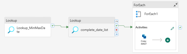
Here is the complete pipeline orchestration
Best Practices and Optimization Tips
1. Monitor and Adjust Parallelism
By default, Fabric will run multiple ForEach iterations in parallel based on your capacity. For F64 capacity (common trial size), you might see 10-15 parallel executions. Keep an eye on:
- Source database load too many parallel queries can overwhelm smaller databases
- Pipeline execution time if everything finishes in 5 minutes, you might be over-partitioned
2. Handle Failed Partitions Gracefully
Sometimes individual partitions fail due to transient issues. Consider adding:
- A logging table to track which partitions succeeded/failed
- Retry logic on the Copy Activity (set Retry count to 2-3)
- A separate pipeline to reprocess only failed partitions
3. Consider Incremental Loads
Once your initial historical load is complete, you probably don’t need to reload everything every day. Instead:
- Modify your MinMaxDate query to only look at recent dates (e.g., last 15 days)
- Use parameters to pass in start/end dates for incremental processing
4. Use Metadata-Driven Pattern for Multiple Tables
If you have dozens of fact tables to load, create a control table with metadata:
CREATE TABLE control.LoadMetadata (
TableName VARCHAR(100),
PartitionColumn VARCHAR(100),
DestinationPath VARCHAR(200),
IsActive BIT
);
Then add an outer ForEach loop that reads from this control table and calls your partition pipeline for each active table. This is exactly the pattern Microsoft recommends in their latest metadata-driven pipeline documentation.
Conclusion
Source query limits are a structural reality in enterprise data environments. Designing pipelines that respect those limits while still delivering complete datasets is part of building a mature data platform.
Partition-based loading in Microsoft Fabric provides a repeatable and scalable pattern that can be extended to multiple tables, environments, and future growth scenarios. Once implemented correctly, it becomes a foundational capability rather than a workaround.
In modern data platforms, resilience is not achieved by removing constraints. It is achieved by designing systems that work intelligently within them.