In Part 1 of our Inforiver series, we explored how to streamline operational expense forecasting by moving beyond traditional spreadsheets to a more integrated approach within Power BI. Now, in Part 2, we’ll shift our focus to sales forecasting, one of the most critical yet challenging aspects of financial planning.
Sales forecasting involves multiple variables that can significantly impact revenue projections: seasonal trends, market conditions, product mix changes, and most importantly, pricing strategies. Traditional forecasting methods often struggle to handle these complexities effectively, especially when finance teams need to model different price scenarios or adjust for dynamic market conditions.
The challenge becomes even more complex when you need to account for price changes across different products, regions, or time periods. Finance teams typically find themselves juggling multiple spreadsheets, struggling to maintain consistency across scenarios, and spending countless hours on manual calculations that could be automated.
Inforiver Writeback Matrix transforms this process by enabling sophisticated sales forecasting directly within Power BI, complete with dynamic pricing adjustments and scenario modeling capabilities. Unlike static reporting tools, Inforiver allows you to interact with your data, modify assumptions in real-time, and immediately see the impact on your forecasts-all while maintaining the familiar spreadsheet-like interface that finance professionals prefer.
This approach eliminates the disconnect between reporting and planning, ensuring your sales forecasts become an integrated part of your data ecosystem rather than isolated spreadsheet files that quickly become outdated or inconsistent.
What You’ll Learn
In this comprehensive guide, you’ll master the essential skills needed to transform your sales forecasting process using Inforiver Writeback Matrix. By the end of this tutorial, you’ll be able to:
- Create dynamic sales forecasts based on historical performance data and trends
- Modelling the impact of price adjustments on volume and revenue forecasts
- Modify forecast assumptions directly within Power BI using intuitive grid-based editing
- Distribute forecast values proportionally across products, regions, or time periods
- Write back finalized forecasts to your Microsoft Fabric Warehouse for enterprise-wide access
Practical Application:
We’ll demonstrate these capabilities using a realistic sales forecasting scenario that includes multiple product lines, and strategic price adjustments. This hands-on example will show you how to handle real-world complexities while maintaining the simplicity and efficiency that makes Inforiver so powerful for financial planning teams.
This tutorial builds upon the foundational concepts from Part 1, so you’ll be leveraging the same powerful writeback capabilities while exploring more advanced forecasting features specifically designed for revenue planning and price optimization.
Let’s start with a Sales Model built on Contoso data. In this model, we will forecast for Y months, while X months represent actuals. Here, X refers to past months, and Y includes the current and upcoming months. For example, if the current month is October, actual sales will cover January to September, and forecasts will be generated for October to December. The forecast will be based on the same months from the previous year- specifically, we will project sales as 1.5 times last year’s volume for the corresponding month. This forecast will be on volume, which we will then multiply by price to derive the revenue forecast.
To support this, we will require the following measures in our model:
- Actual Sales
- Volume
- Budget Volume (last year same month volume × 1.5)
- Price
Step 1: Set up Inforiver visual:
1. First, add the Inforiver Writeback visual to the report canvas and add the necessary fields to the visual.
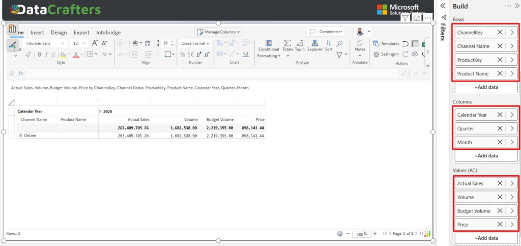
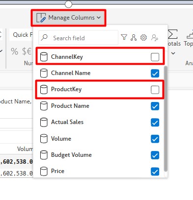
2. Then hide the unnecessary columns using the Manage Columns option.
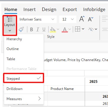
3. Make the layout Stepped from Layout options under the Home tab.
Since our target is to create a volume forecast and then multiply it by Price to get the revenue forecast, first we set up the volume forecast, then we will create price input functionalities, and finally we will create the revenue forecast.
Step 2: Create Volume Forecast Measure:
To create volume forecast measure,
1. Navigate the Insert tab → Forecast Measure
2. Fill in the following fields and click Next:
- Measure Name: Volume Forecast
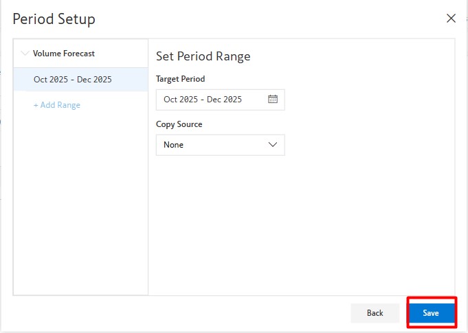
- Forecast Period: Oct 2025-Dec 2025
- Close Period: Measure
- Linked Measure: Volume
- Open Period: Data Input
- Default Value: Measure
- Measure: Budget Volume
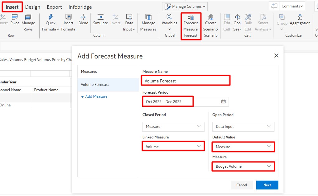
3. The Period Setup should be left as it is, and select the Save button.
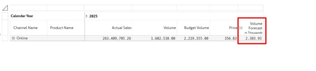
4. Now you can see the volume forecast measure in the visual.
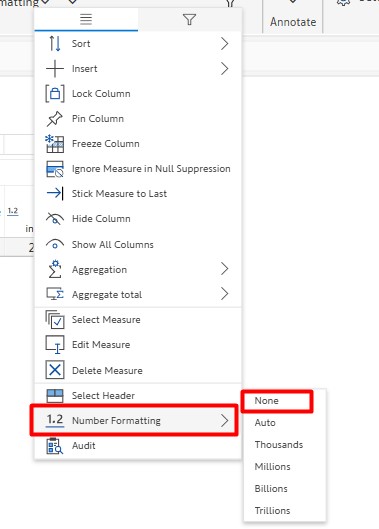
5. Formatting: Right-click the measure → Number Formatting → None.
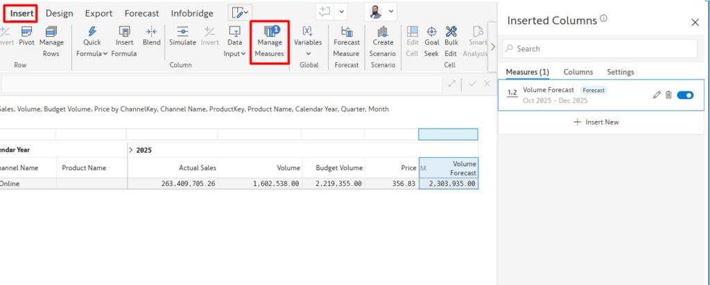
6. To reduce decimals:
- Go to Insert tab → Manage Measures → select Volume Forecast.
- By selecting the measure from the Home tab, use Decrease Decimal.
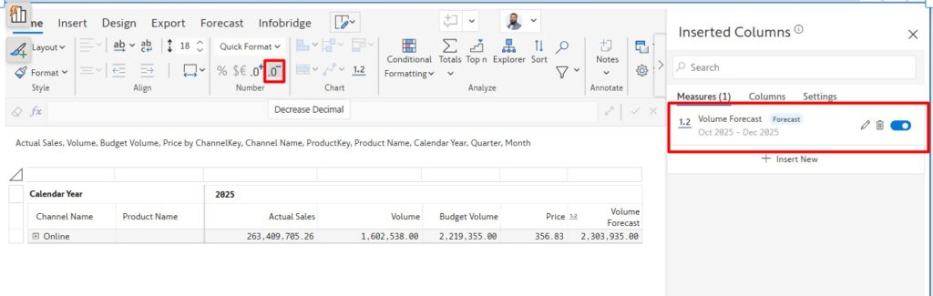
7. Since we already have the Volume Forecast measure, we don’t need the Budget Volume measure in the visual anymore. So, hide the measure using the Manage Columns options.
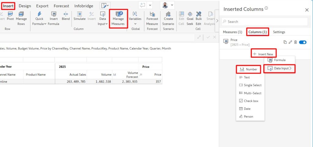
Step 3: Create Price Column
1. Go to Insert tab → Manage Measures.
2. Under Columns, choose Insert New → Formula → Number.
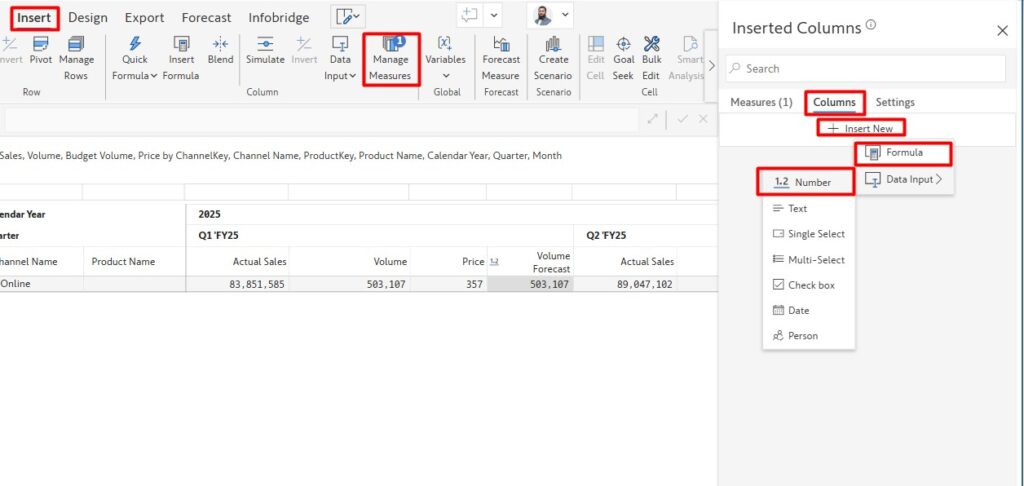
3. Now fill up the Formula Measure fields and click the Create button:
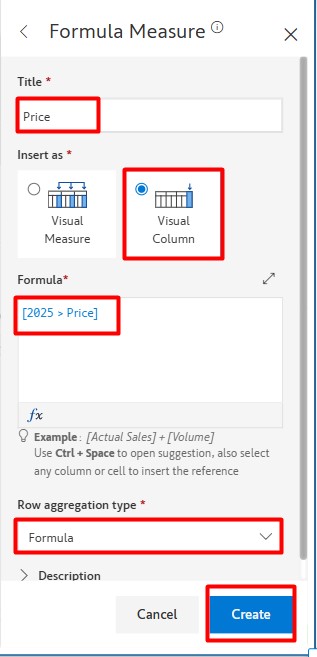
- Title: Price
- Insert as: Visual Column
- Formula: [2025>Price]
- Row Aggregation Type: Formula
4. Rename the column header to Price (double-click header).
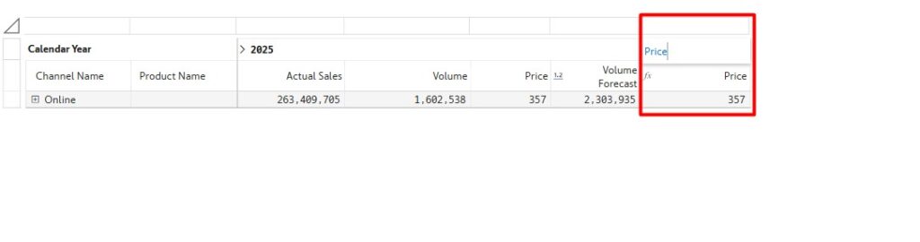
5. Hide the original Price column from Manage Columns.
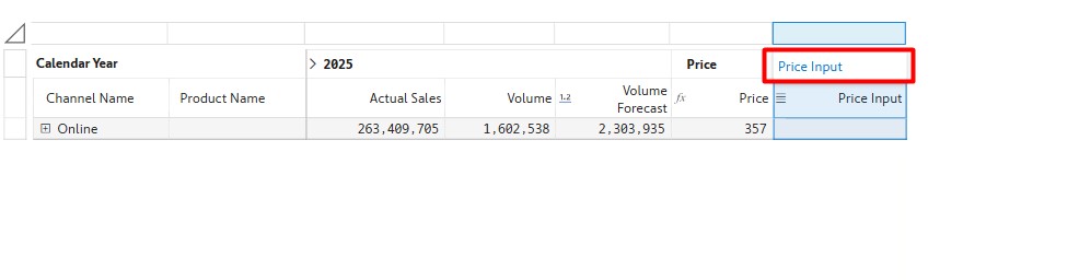
Step 4: Create Price Input Column
Now we will create a new blank Price Input column to input new prices when needed. We don’t overwrite the price in the existing Price column because after overwriting the previous value, we can’t track it. That’s why, to keep both the old and new Input Price in the visual to show at the same time, we are creating a separate price input column.
1. Repeat the same process as creating the Price column.
2. This time, select Data Input instead of Formula.
2. Fill in the following fields and click on Create button.
- Title: Price Input
- Insert as: Visual Column
- Input type: Number
- Row aggregation type: Average (Leaf)
- Distribute parent value to children: Enable
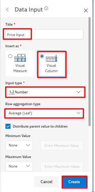
3. Rename the column header to Price Input.
Step 5: Create Revenue Forecast Measure
Since we now have Volume Forecast and Price information in the visual, we will create the Revenue Forecast now.
1. Go to Insert tab → Forecast Measure.
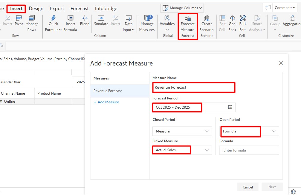
2. Fill in the following:
- Measure Name: Revenue Forecast
- Forecast Period: Oct 2025-Dec 2025
- Close Period: Measure
- Linked Measure: Actual Sales
- Open Period: Formula
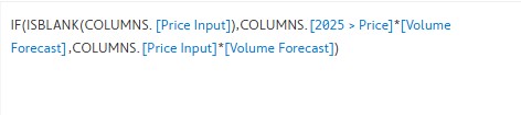
- Formula:
IF(
ISBLANK(COLUMNS.[Price Input]),
COLUMNS.[2025>Price] * [Volume Forecast],
COLUMNS.[Price Input] * [Volume Forecast]
)
3. Format the measure (remove decimals, set plain number) the same way as Volume Forecast.
Step 6: Hide Forecast Measures for Closed Periods
If you expand the columns from year level to quarter level, you can see the Volume Forecast and Revenue Forecast measures are also in the previous periods. Since we only need these measures for open periods (Oct 2025 to Dec 2025), we need to hide the measures for the closed period.
- Go to Home tab → Click dropdown icon beside the Hide icon→ Hide closed periods.
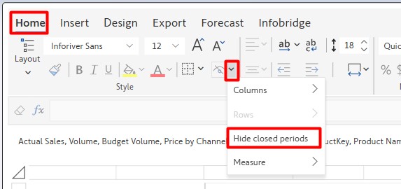
After hiding Forecast measures for the closed period, you can see Actual Volume and Sales for the closed period and Forecast Volume and Revenue for open periods.
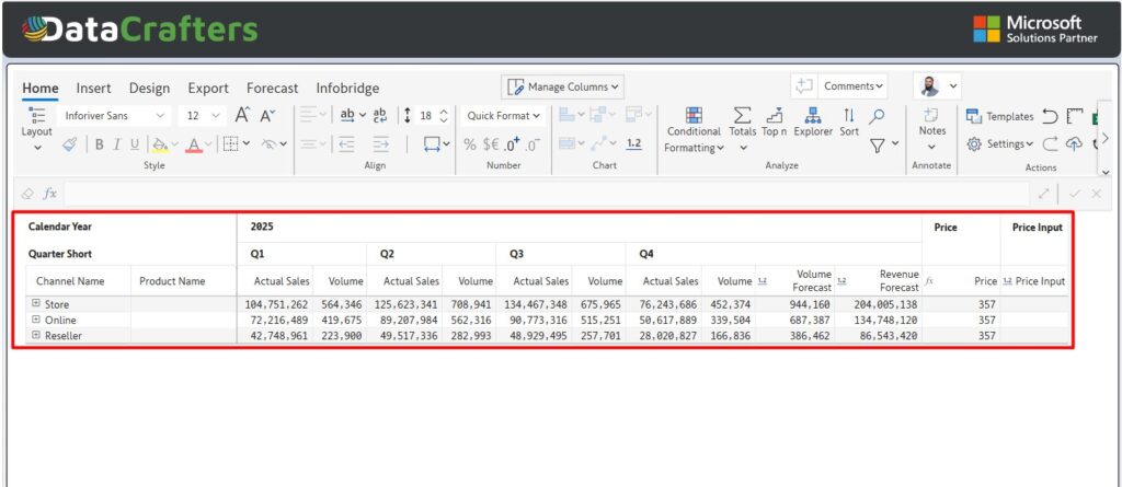
By following the above steps, you can forecast numbers using Inforiver Writeback Matrix.
Now if you want to write back those forecast data to Lakehouse/Warehouse for further use, please follow the Step 5 from the part 1 blog of this series or follow the official documentation from Inforiver [https://docs.inforiver.com/working-with-inforiver/12.-data-writeback].